OPENCoastS is an online service that assembles on-demand circulation forecast systems for selected areas and keeps them running operationally for a period defined by the user. This service generates daily forecasts of water dynamics variables (water levels, velocities, temperature, salinity, wave parameters) over the region of interest for 48 hours, based on numerical simulations of all relevant physical processes. Presently, all forecasts are made with the model SCHISM (http://ccrm.vims.edu/schismweb/), version 5.4.1.

The service is accessible at https://opencoasts.ncg.ingrid.pt/ supported by the computational resources from INCD - Infraestrutura Nacional de Computação Distribuída (https://www.incd.pt), a node of the EGI - European Grid Infrastructure (https://www.egi.eu), and from IFCA - Institute of Physics of Cantabria (https://ifca.unican.es).

Access to the service is granted through a registration procedure, and is obtained after acceptance of the registration by the OPENCoastS user support team. OPENCoastS is jointly developed and maintained by LNEC - Laboratório Nacional de Engenharia Civil (LNEC - http://www.lnec.pt), LIP - Laboratório de Instrumentação e Física Experimental de Partículas (LIP - https://www.lip.pt), CNRS-LIENSs - Centre National De La Recherche Scientifique - LIttoral ENvironnement et Sociétés (CNRS-LIENSs - https://lienss.univ-larochelle.fr) and Universidad de Cantabria (UC - https://web.unican.es).

Three types of forecast systems are available, depending on the physical processes being solved:

1) 2D barotropic simulations without short waves - these simulations are fast and provide water levels and depth-averaged velocities as outputs. Forcings include tides, wind, atmospheric pressure and river flow. They can be applied anywhere in the world. This is the recommended option for a first deployment at a site.

2) 2D barotropic simulations with wave-current interaction - these simulations provide wave parameters besides the ones in the option above. Wave-current interactions are simulated and forcings include short waves besides the ones above. The region where this option can be used is limited to the North Atlantic area, as the wave boundary conditions are limited to this area. This option should only be selected at sites where short waves are relevant as computational costs are considerably larger than option 1. A first deployment with option 1 is advised.

3) 3D baroclinic simulations - these simulations provide 3D fields of velocity, salinity and temperature, besides water levels. They can be forced by tides, river flow and temperature and salinity at all the boundaries, besides the atmospheric forcing (wind, air temperature, pressure, humidity, solar radiation and downwelling longwave radiation) at the surface. These forecasts can be generated anywhere in the world. The full baroclinic equations are used. Thus, they are quite demanding computationally and more complex to set-up with success. Unlike the previous options, that are freely available to all, access to these simulations is granted on request (send an email to aoliveira@lnec.pt for access).

This manual presents a detailed guide to help users use the OPENCoastS service under these 3 options. In particular, it helps the user to take advantage of the service’s three main features:

Configuration Assistant: this feature guides the user in the process of creating a new forecast system at the user’s region of interest, following 6 simple steps. It only requires the availability of a computational 2D unstructured grid in the SCHISM/ADCIRC/SELFE format (SCHISM v5.6 manual, pages 52-54). For 3D baroclinic runs the user must also provide a vertical grid file (SCHISM v5.6 manual, pages 54-56).

Figure 1 - Configuration Assistant page preview

Forecast Systems: this feature allows users to manage their forecast systems, through a number of tasks that can be done on a forecast system, e.g.: edit the system’s configuration at any time before submission, delete it, clone it, generate a print-preview, activate (submit) / deactivate it or request an extension of the forecast’s duration.

Figure 2 - Forecast System Manager page preview

Outputs Viewer: this feature allows the user to visualize the daily predictions for each forecast and to compare model predictions with available EMODnet monitoring stations.

Figure 3 - Output Viewer page preview

Registration and Login

To be able to start using the service, a new user must first register:

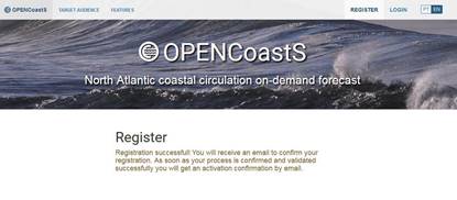
Figure 4 - Preview of OPENCoastS register page

As an alternative, users can register through the EGI check-in service using their affiliation entity identification:

Figure 5 - Preview of the EGI Check-in service

Figure 6 - OPENCoastS message on new user registration

After registering a confirmation is issued at the site and a confirmation email is sent to the user:

Figure 7 - OPENCoastS email text sent on new user registration

The user must then confirm the registration through the link provided in the registration acknowledgement email.

Note: If the registration is made via EGI, no confirmation is required.

With this confirmation, a validation request is launched and as soon as this request is validated and accepted, an email is sent confirming the access to the service. From that point onward, the user can login and start using the OPENCoastS service.

Figure 8 - Preview of OPENCoastS login page

Note: Users can at any time request a new password, in case they have forgotten it, by clicking on the “Forgot my password” link and providing their user email.

After login in for the first time, the user is prompted to accept the Terms and Conditions. This acceptance is necessary to be able to use the service.

Figure 9 - Preview of the Terms and Conditions of the service usage

After accepting these terms, the user is ready to start deploying forecasts and is automatically taken to the Configuration Assistant.

Configuration Assistant

First time usage

The first time a user enters the Configuration Assistant, a guided tour on the assistant is proposed. The user can skip it by hitting the “close” button at any time or can follow it back and forth through the guide’s steps. All steps have a button that opens this guide with tips on how to use each step.

Figure 10 - Previews of the Configuration Assistant Guide

Next to the button all steps also have the button that opens a collapsible panel with a more detailed description of each step.

Figure 11 - Detail of a step's detailed description collapsible panel

The Header indicates in which step the user is at the Configuration Assistant and also can be used for navigating between available steps. Most steps require users to fill out forms with mandatory fields. They can then move to the next step by clicking the “Complete step” button which will validate the user’s choices. Users can also move back and forward through the steps clicking on the “Previous” and “Next” buttons or reset the current step by clicking the “Restart step” button. Note that resetting a step implies also resetting the steps ahead already completed for they are sequentially dependent on each other.

Users should save the forecast system at an early stage and along the process in order to avoid loss of information, by using the “Save” button (top right screen) and providing a name for the system on the first time it is saved. The service will assign a forecast ID number to each forecast system. Users can then access each forecast deployment using the “Forecast Systems” page and re-open it on the Configuration Assistant, if the system is still under configuration.

Next to the “Save” button is the “New System” button that resets entirely the Configuration Assistant. Note that in order to not loose work already done on a system’s configuration, the user must first save it.

Attention: changes to a step already completed require the user to click the step’s “Save changes” button, located at the bottom of the page, in order to re-validate the step and save the changes.

Creating a new forecast system

The creation of a new forecast system requires following 7 steps:

Step1: In this step the user will choose the run type (2D Barotropic, 3D Baroclinic or 2D Waves & currents), the model to use and the daily forecast range. Presently, only version 5.4.1 of the SCHISM model is available and the forecast range is limited to 48 hours.

Step2: In this step, the user has to provide computational grids for the forecast in the format adequate for the model chosen in the previous step. These grids will represent the geographical domain of study. For the 2D barotropic mode and the 2D Waves & currents modes, only an horizontal grid is necessary, along with the indication of the horizontal and vertical Coordinate Reference System of the grid. For the 2D Waves & currents mode, the grid must be in cartesian coordinates. For the 3D baroclinic mode, the user also needs to upload a vertical grid.

Step3: In this step the user has to define the forcing sources for the ocean, river and atmospheric boundaries from the available options.

Step 4: In this step the user selects the stations (virtual sensors) in which time series are extracted with the model output temporal resolution. These can be locations where real time data are available (predefined comparison stations) or other places of interest (virtual stations).

Step 5: For the selected model it is necessary to define all parameters for the simulation. In this step the user will start from predefined parameter files and can change some of their parameters, if needed.

Step 6: In this step the user can define additional parameters of the model, by specifying constant values or uploading files with spatially variable values.

Step 7: Confirms the selected configurations and activates the forecast system.

Building a forecast system step by step

Step 1 - Model

In this configuration step the user selects the run type, the model version to use in the forecasts, as well as the forecast range (in the present version ‘48h’ is the only available option). The run type options are between: 2D Barotropic, 3D Baroclinic (available only to users with advanced permissions) and 2D waves & currents.

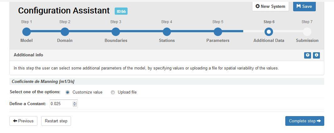
Figure 12 - Preview of Step 1 - Model

The OPENCoastS platform uses the circulation model SCHISM (Zhang et al., 2016), that solves the shallow water equations. SCHISM is a community model, based on unstructured grids and fully parallelized, that simulates a vast range of processes in water bodies. SCHISM simulates thus water levels and velocities due to tides, wind, atmospheric pressure and river flow, in 2D depth-averaged mode. Presently, only version 5.4.1 of the SCHISM model is available in this service.

For 3D Baroclinic runs the SCHISM model simulates other variables, such as temperature and salinity.

For the 2D waves & currents option, the model WWM (Roland et al., 2012) will be activated within SCHISM. WWM is a spectral wave model that simulates the generation and propagation of short waves. It is coupled to the SCHISM model in order to provide radiation stresses that affect circulation, and to receive water levels and velocities.

After filling in the required fields, the user can move to the next step pressing the “complete step” button.

References and links useful for this step:

● Zhang, Y.J.; Ye F.; Stanev, E.V.; Grashorn, S., 2016 – Seamless Cross-scale Modeling with Schism. Ocean Modelling, 102: 64-81.

● Roland, A., Zhang, Y., Wang, H.V., Meng, Y., Teng, Y., Maderich, V., Brovchenko, I., Dutour-Sikiric, M. and Zanke, U. (2012) A fully coupled wave-current model on unstructured grids, Journal of Geophysical Research-Oceans, 117, C00J33, doi:10.1029/2012JC007952.

● SCHISM URL: http://ccrm.vims.edu/schismweb/

Step 2 - Domain

In this step the user must upload a simulation grid (“horizontal grid”) in a format compatible with the model chosen in the previous step. For the SCHISM model the grid should be in the “hgrid.gr3” or “hgrid.ll” format (see SCHISM manual). This format is also used in other coastal models, such as ADCIRC, ELCIRC or SELFE. These grids can be built with grid generators such as XMGREDIT or SMS, among other tools.

Note that although SCHISM allows the use of hybrid grids, composed of triangles and quadrangles, the OPENCoastS service only works with triangular grids. The service also limits the size of uploaded files (17 MB) and the maximum number of nodes in the grid (175 000 nodes), in order to allow access to more users and a sustainable usage of the infrastructure.

For 3D Baroclinic runs the user must also provide a vertical grid file as input. For format, see SCHISM manual.

The user must also indicate the “Coordinate Reference System” of the grid, from a list of predefined systems available or in alternative specifying an EPSG code (more info on codes EPSG) and provide the “Vertical reference” of the grid to allow a correct comparison with real time data available at the region of study and a correct specification of boundary conditions. The user can select from the Hydrographic Zero or Cascais height, or establish his own vertical displacement relative to Mean Sea Level. When this reference is unknown, the user can enter the value 0 as reference. Note that in the 2D waves & currents option, a cartesian coordinate system must be selected in this version.

Optionally, the service also allows the estimation of an adequate “time step”, based on the analysis of grid resolution, i.e., the dimension of its elements. It searches for a maximum Courant number below 100.

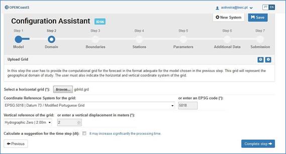
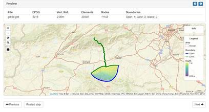
Figure 13 - a) Preview of Step 2 - Domain for a 2D deployment; b) Preview of Step 2 - Domain for a 3D deployment

The completion of this step validates the uploaded grid and the EPSG choice. If the file is not valid, the user gets an error message. If validation fails to apply a coordinate conversion, the user is prompted to select a different coordinate reference system (EPSG). If the file is valid and the selected EPSG is applicable, the user is redirected to an intermediate step where he/she can confirm visually on the map if the processing of the computational domain and its bathymetry is correct.

Figure 14 - Details on Step 2 validation (1: coordinate conversion prompt message example; 2: incorrect EPSG selection example)

If this is not the case the user must click on the “Restart step” button in order to upload a new grid file or choose a different EPSG code.

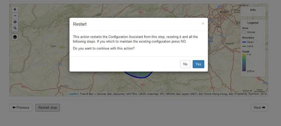
Figure 15 - Details on Step 2 - restarting / resetting step

If all is in order the user just has to click “Next”.

Figure 16 - Details on Step 2 - grid valid and ready for next step

Step 3 - Boundaries

This step allows users to select the type of forcing to be used at each boundary of the simulation grid (ocean or river) and over the domain (atmospheric).

Regarding the open boundaries of the model, the present version of OPENCoastS service allows the following options for ocean boundaries:

Water levels

● PRISM2017 - Portuguese Regional Tide-Surge Model Forecasts 2017

● FES2014 - last (2014) version of the FES (Finite Element Solution) global tide model

● CMEMs global - global 3D circulation model

● CMEMs IBI - Iberian shelf 3D circulation

2. Temperature and salinity

● CMEMs global - global 3D circulation model

● CMEMs IBI - Iberian shelf 3D circulation

The PRISM2017 forecast system is developed and operated by LNEC to forecast water levels along the Portuguese coast. PRISM2017 simulates tides and storm surges in NE Atlantic using model SCHISM in 2D and barotropic mode. The model is forced by global tidal model FES2012, tidal potential, atmospheric pressure and winds from model GFS. The resolution of the grid for the Portuguese coast is in the order of 250 m. More info on model implementation and validation can be consulted in Fortunato et al. (2016) and Fortunato et al. (2017). Note that, when simulations are forced by PRISM2017 results, only water levels are imposed at the boundaries. This simplification can lead to spurious velocities at the boundaries.

FES2014 is the latest version of the FES (Finite Element Solution) tide model developed in 2014-2016. It is the improved version of the FES2012 model. This new FES2014 model has been developed, implemented and validated by the LEGOS, NOVELTIS and CLS, within a CNES funded project. FES2014 takes advantage of longer altimeter time series and better altimeter standards, improved modeling and data assimilation techniques, a more accurate ocean bathymetry and a refined mesh in most shallow water regions. Special efforts have been dedicated to address the major non-linear tides issue and to the determination of accurate tidal currents. FES2014 is based on the resolution of the tidal barotropic equations (T-UGO model) in a spectral configuration. A new global finite element grid (~2.9 million nodes, 50% more than FES2012) is used and model physic has been improved, leading to a nearly twice more accurate 'free' solution (independent of in situ and remote-sensing data) than the previous FES2012 version. Then the accuracy of this 'free' solution was improved by assimilating long-term altimetry data (Topex/ Poseidon, Jason-1, Jason-2, TPN-J1N, and ERS-1, ERS-2, ENVISAT) and tidal gauges through an improved represented assimilation method. Details are presented in Carrere et al (2016). Note that if FES2014 is selected, and atmospheric forcings are imposed, then an inverse barometer effect is imposed at the ocean boundaries, superimposed on the tidal elevation signal.

The Copernicus Marine Service (CMEMS) provides observation-based and forecast-based information about the state of the and regional seas. Two products from CMEMS are available in OpenCoastS: i) the global ocean analysis and forecast system (GLOBAL_ANALYSIS_FORECAST_PHY_001_024; https://resources.marine.copernicus.eu/?option=com_csw&task=results?option=com_csw&view=details&product_id=GLOBAL_ANALYSIS_FORECAST_PHY_001_024) and ii) the IBI (Iberian Biscay Irish) ocean analysis and forecasting system (IBI_ANALYSIS_FORECAST_PHYS_005_001; https://resources.marine.copernicus.eu/?option=com_csw&task=results?option=com_csw&view=details&product_id=GLOBAL_ANALYSIS_FORECAST_PHY_001_024).

The Operational Mercator global ocean analysis and forecast system provides 10 days forecasts of 3D global hydrodynamic conditions and is updated daily. The global ocean information is available with a 1/12º horizontal resolution with regular longitude/latitude equirectangular projection. Regarding the vertical grid, 50 vertical levels ranging from 0 to 5500 meters are available. This product includes, among others, daily mean fields of temperature and salinity and hourly mean surface fields for sea level height, which are used in the OPENCoastS service. Further information about the product is available in Chune et al. (2019) - https://resources.marine.copernicus.eu/documents/PUM/CMEMS-GLO-PUM-001-024.pdf - and Lellouche et al. (2019) - https://resources.marine.copernicus.eu/documents/QUID/CMEMS-GLO-
QUID-001-024.pdf.

The operational IBI (Iberian Biscay Irish) ocean analysis and forecasting system is a regional application that provides a 5-day hydrodynamics forecasts and is updated daily. The system is based on an application of the NEMO model using a horizontal grid with 1/36º resolution. Regarding the vertical grid, 50 vertical levels ranging from 0 to 5500 meters are available. This product includes 6 different datasets, among which 3D daily means fields of temperature, salinity and hourly mean sea surface height, which are used in the OPENCoastS service. Further information about the product is available in Amo et al. (2019) - https://resources.marine.copernicus.eu/documents/PUM/CMEMS-IBI-PUM-005-001.pdf - and Sotillo et al. (2019) - https://resources.marine.copernicus.eu/documents/QUID/CMEMS-IBI-QUID-
005-001.pdf.

Figure 17 - Preview of Step 3 – Boundaries and detail of the Popup form

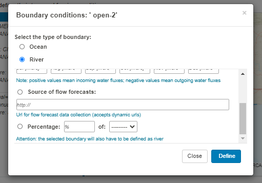
To specify the required Boundary conditions, the user must select each boundary by ticking its corresponding checkbox in the table (on the left) and then click on the “Define type and forcing condition” button. This will open a popup form where the user must choose between an ocean or a river boundary. If several boundaries are selected at the same time, then the specified values will be applied equally to all of them.

For the ocean boundaries the users must still select a forcing source to apply to all ocean boundaries. The several options are available in a pull-down below, for water levels and for salinity and temperature in the 3D version.

Figure 18 – Selection of the source of ocean boundary conditions

For the river boundaries the users must define manually, from the popup form (Figure 19), the monthly average river flow in m³/s (climatology) of each river boundary or a fixed value for the whole simulation. The same applies to temperature and salinity for the 3D runs. Positive river flows values are considered as incoming water fluxes and negative values as outgoing water fluxes.

For the river boundaries where flow predictions are available it is possible to upload a permanent link where the prediction of river flow can be collected by OPENCoastS. The format is an ASCII format, following the indication in pag 65 of SCHISM’s manual: http://ccrm.vims.edu/schismweb/SCHISM_v5.3.1-Manual.pdf (4.3.1 Optional inputs: .tc (ASCII)). Another alternative is to set the river flow as a percentage of another river flow boundary.

Figure 19 - Detail of the Popup Form to define river boundaries forcing conditions for URL or percentage options.

The user finally must select the atmospheric forcing for the forecast system (or select not to use atmospheric forcings). Currently, the NOAA and Arpege atmospheric forecasts are available for the 2D deployments but for 3 forecasts, only NOAA’s outputs can be used, as it is the only provider that has all necessary inputs for the 3D run. The Arpege forecasts only cover the European coasts.

Figure 19 - Detail of the Popup Form to define river boundaries forcing conditions

Figure 20 - Preview of Step 3 – Boundaries, all filled out for a) a 2D run and b) a 2D W&C runs.

References and links useful for this step:

● Carrere L., F. Lyard, M. Cancet, A. Guillot, N. Picot: FES 2014, a new tidal model - Validation results and perspectives for improvements, presentation to ESA Living Planet Conference, Prague 2016.

● Fortunato, AB; Li, K; Bertin, X; Rodrigues, M; Miguez, BM. 2016. Determination of extreme sea levels along the Iberian Atlantic coast, Ocean Engineering 111, 1: 471 - 482. doi: 10.1016/j.oceaneng.2015.11.031

● Fortunato, AB; Oliveira, A; Rogeiro, J; Tavares da Costa, R; Gomes, JL; Li, K; de Jesus, G; Freire, P; Rilo, A; Mendes, A; Rodrigues, M; Azevedo, A (2017). Operational forecast framework applied to extreme sea levels at regional and local scales, Journal of Operational Oceanography, 10/1: 1-15. doi: 10.1080/1755876X.2016.1255471

● http://www.umr-cnrm.fr/spip.php?article121&lang=en

● Amo, A.; Reffray, G.; Sotillo, M.G.; Aznar, A.; Guihou, K. (2019). Atlantic -Iberian Biscay Irish- IBI Production Centre IBI_ANALYSIS_FORECAST_PHYS_005_001. Product User Manual. Issue 6.2. CMEMS, 47 pp.

● Chune, S.L.; Nouel, L.; Fernandez, E.; Derval, C.; Tressol, M. (2019). GLOBAL Ocean Sea Physical Analysis and Forecasting Products GLOBAL_ANALYSIS_FORECAST_PHY_001_024. Product User Manual. Issue 1.5. CMEMS, 35 pp.

● Lellouche, J.-M.; Legalloudec, O.; Regnier, C.; Levier, B.; Greiner, E.; Drevillon, M. (2019). Global Sea Physical Analysis and Forecasting Product GLOBAL_ANALYSIS_FORECAST_PHY_001_024. Quality Information Document. Issue 2.1. CMEMS, 81 pp.

● Sotillo, M.G.; Levier, B.; Lorente, P.; Guihou, K. (2019). Atlantic-Iberian Biscay Irish- IBI Production Centre IBI_ANALYSIS_FORECAST_PHYS_005_001. Quality Information Document. Issue 4.1. CMEMS, 107 pp.

Step 4 - Stations

This step allows establishing locations where to extract model time series with the model output resolution, for automatic comparison of predictions with real-time stations, or to get time series at user-selected locations (virtual sensors). The system automatically identifies the available real-time stations available in the computational domain of the grid (observation stations from those available at EMODnet) and proposes them in the table (limited to 5 stations). This step is optional and if the user does not want these predefined outputs he/she only has to complete the step without interaction.

Figure 21 - Preview of Step 4 - Stations

The user can add new stations by clicking the button “New Station” or by clicking directly on the map. These actions will open a popup form with the difference being that the station’s position coordinate is already pre-filled if the user clicks on the map. Note that the new station’s position must be placed inside the domain (grid) area. From the form user must choose between “Comparison” and “Virtual” type of station and fill out the mandatory fields.

The Comparison Station will use data from observation stations as a reference of comparison with the new station’s values. The chosen observation station may be located outside of the domain. If the distance between points is above the recommended (100 meters) the user will be notified in the form. However, it can still be created; this notification is only a warning.

If the location of the comparison station does not match the exact location of the observation station, a line will be created linking both visually.

The Virtual Station requires the user only to fill in a name describing the station. In this case no comparison is made to the extracted time series data at the specified location.

Figure 22 - Details of Step 4 (1: the New Station Popup Form; 2: after adding new comparison and virtual stations, 3 - wave and current simulation)

The user can remove added stations permanently by clicking on them on the map and on the button “Remove” or just deselect them, in this case they remain in the table and can be selected at any time whilst the forecast system is still in the configuration stage.

Step 5 - Parameters

In this step the user can opt to use the predefined parameters proposed by the OPENCoastS service used in model SCHISM or configure the available parameters for edition. In this current version only a few parameters are available for edition, e.g., the time step (dt) or the model ramp period (dramp).

Based on the parameters defined here, the parameter file (param.in) is automatically created for use in the SCHISM model (for more information see SCHISM’s user manual - http://ccrm.vims.edu/schismweb/SCHISM_v5.6-Manual.pdf). Future versions of the service will allow the user to upload directly a param.in file, fully edited and created by the user.

Figure 23 - Preview of details on Step 5 – a) Parameters for a 2D run; b) Parameters for a 3D run; c) Parameters for 2D Waves & Currents

Step 6 - Additional Data

This step allows the user to define the additional parameters not defined in param.in. In the current version, only the Manning coefficient is available for the 2D deployments (with or without waves). This coefficient is used by the SCHISM model in 2D mode to determine bottom friction based on local characteristics. The user can specify a constant value or, in alternative, upload to the system a file with the spatial variation of this value (grid format - .gr3). The Manning coefficient is defined in m^1/3/s.

For the 3D deployments several parameters need to be defined, within a predefined range.

Figure 24 - Preview of Step 6 - Additional Data a) 2D run; b) 3D run

Step 7 – Submission

In this step the user can review a summary of all configured steps as well as submit / activate the forecast system. The activation of the system will launch the forecast system in the computational infrastructures available. Currently, the simulations will be carried out using the INCD – Portugal’s National Infrastructure for Distributed Computing and IFCA (Spain) facilities.

Figure 25 - Preview of Step 7 - Submission

By selecting a Step on the left panel, a summary of that step unfolds revealing the user’s selections along the configuration stage. Some steps provide additional functions, e.g. the Domain and Parameters steps allow users to download the domain grid and the param.in files, respectively.

Note: if the uploaded horizontal grid on Step 2 contained projected coordinates, the user can download the original uploaded file (.gr3) and also the grid file converted to geographic coordinates WGS84 (.ll).

Users can save the configured forecast system (press the “Save” button on the top right screen) and submit later on at any time.

To submit and launch the forecast system, the user must first accept the Terms and Conditions of Use, provide a “Name” for the system (if not done previously) and optionally add a brief “Description” to it and finally press the “Activate System” button.

$Text Box: Figure SEQ Figure \* ARABIC 26 - Details on Step 7 - Submission; 1: domain preview and files download; 2: filling the submission form$

This action will redirect the user to the “Forecast Systems” page where the system in question will switch from the “Configured” to the “Active” status . An active forecast system can also be referred as a deployment. The first simulations will start the following day.

Figure 27 - Details on Step 7 - Submission; after activating a forecast system

Forecast Systems

Monitoring my forecasts

The Forecast Systems page allows users to monitor and manage their forecast systems. It provides an overview of their state and helps to anticipate the need for time extensions and to remove unwanted systems or deployments (submitted systems) that are not well configured or already expired.

Figure 28 - Preview of the Forecast Systems page

Each user will only be able to see their own deployments. Only people assigned with “Administrator” permission are allowed to see other deployments.

Managing forecast systems

Configuration mode

Once a forecast system is created and saved, the user can logout and continue the configuration later on. The “Open System” tool allows the user to continue this task at its own pace. Until the system is launched, the configuration is open for changes.

Figure 29 - Opening a system on the Configuration Assistant

After clicking on this tool, the Configuration Assistant opens, loads the selected system and allows the user to continue to set up the selected system under configuration.

Deleting a forecast system

If a forecast system is not necessary any longer, the user can eliminate it (saving resources and allowing for the setup of a new system if their system’s quota has been reached).

By clicking on the “Delete System” tool the system is erased. Note that access to results will be lost and this forecast cannot be recovered. Also, the delete tool is not available for deployments in the “Active” state. Deployments must be deactivated before they can be deleted.

As for other actions, an acknowledgement of the deletion is provided.

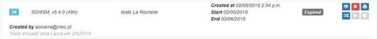
Figure 30 – Details on deleting a system

Print preview

By pressing the “Print Configuration” tool the user opens a report of the forecast system’s configuration summary on a new page for printing purposes. This option is available as soon as the system is configured.

Figure 31 - Printing a system's report

Reviewing a deployment’s configuration

Activated/submitted forecast systems present a different toolbar from those still in configuration. When the system is activated, it can no longer be configured, so, the “Open System” is replaced with the “View Configuration” tool which opens a modal panel presenting the forecast system’s configuration summary for reviewing purposes, along with its tools.

Figure 32 - View deployment's configuration summary

Cloning a forecast deployment

This tool was developed to facilitate the creation of new deployments that only have marginal changes relative to operating ones. If the user presses the “Clone System” tool the service duplicates the deployed forecast system in question into a new system, still in the configuration stage.

Cloned systems are issued an ID number that refers to the number of the one from which it was created, i.e., the original deployment; e.g. “62:57” where 62 is the ID of the new system and 57 the ID of the original deployment.

Figure 33 - Details on cloning a deployment

Once the clone is created, the user can press its “Open“ tool, being redirected to the Configuration Assistant. Then navigate to the step(s) needing adjustments, execute the changes and press the “Change step” button which will re-validate the step and, if valid, save the changes to the step.

After all modifications are done, the user should navigate to Step 7, confirm the changes were applied and launch the new deployment by pressing the “Activate System” button.

Deactivating / activating a deployment

If a deployment is temporarily not necessary, the user can pause it (saving resources and allowing for the setup of a new deployment if the forecast system’s quota has been reached). By clicking on the “Deactivate System” tool, the deployment is paused. Note that access to results will stop.

The system can be restarted by clicking on its “Activate System” button. Note that if the pause is larger than 48 hours, a gap in the prediction stream for that deployment will occur, because the model must be launched in a cold-start mode.

Figure 34 - Details on deactivating / activating a deployment

Extension request

By default, all deployments are set up for one month of operation. If the user wants to extend this period, he/she can click on the “Extend Period” button which will open a form requesting the extension. The request is then evaluated and the user is informed of the decision.

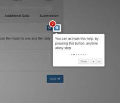
Figure 35 - Extending a deployment’s operation period

Note that the OPENCoastS service adds an “Expiring” label on the Forecast Systems page when a deployment’s operation time is ending, so the user can anticipate the expiration and avoid service interruption. This label is issued one week before expiring.

If the “Expiring” label is red that means it has already entered the 48-hour period and it is no longer possible to continue the deployment without a cold-start on the model. Therefore, the “Extend Period” button is disabled.

Regarding the request form, the user must provide a new limit date as well as the reason supporting this request (as computational resources are limited, a priority must be assigned to deployment extensions).

The request will be acknowledged. Multiple requests to the same deployment are not permitted:

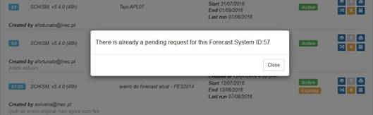
Figure 36 - Details on extending a deployment's operation period

Outputs viewer

The outputs viewer is a simple interface to preview forecast maps and time series at deployment’s comparison and virtual stations. Also, it allows downloading the model results. It provides access to the predictions for each user’s active deployment, under three features: Maps, Stations and Files. While the maps and the stations are available for the latest predictions, the deployment’s files are available for download from the beginning of its activation.

Figure 37 – Viewer feature choice. In the example, the wave peak period is shown in colour and the wave direction in arrows colored with the magnitude of the significant wave height.

The viewer is divided in 3 main panels: on the left a resizable and collapsible menu panel with user’s active deployments and respective tools; on the right a map where user can preview model output (elevations, velocities and other variables) among other tools; in between is a center panel, also resizable and collapsible, where the user can load charts with station time series.

Maps of model predictions

Access to maps of predicted variables is available by selecting the “Maps” button/tab and clicking on the corresponding output map checkboxes. The user can rearrange the order in which the output maps are rendered by dragging their corresponding panel on the Legend Panel (top right screen) and can also change the opacity of each layer and uncover the map’s legend image by clicking on their corresponding label. The following variables can be available, depending on the selected model: Elevation, Velocities (all models), Significant wave height / wave direction, peak period (2D waves & currents model), salinity and temperature (3D baroclinic model).

Figure 38 - Preview of the Outputs Viewer: Maps Feature with layer selection and legend unfolding

On the map’s top left panel is a toolbar that includes multiple functions. Functions include: to zoom in and out; zoom out to the map’s full overview; a toggle tool that allows users to add new output probing stations (that can be seen in time series part of the viewer); a Bookmark menu that allows users to save map bookmarks locally on his/her browser and a Basemap toggle menu from which users can change the map’s basemap. At the bottom of the map, a time slider is also available that allows users to move between the time steps; it also includes a play/pause button to view steps in an animated fashion. Finally, three options are available for the background layer: ESRI World Street Map, ESRI World Grey Canvas, and ESRI World Imagery.

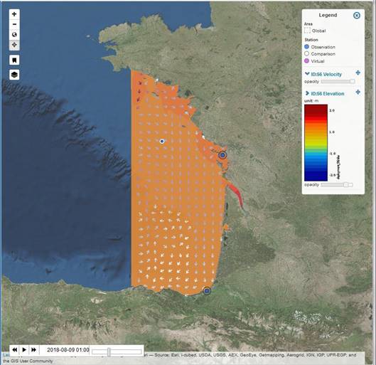
Figure 39 - Maps Feature: functions

Note: the viewer is still under development and may present an erroneous, “inconsistent tiled” behavior. The development team is making the best efforts to overcome these limitations soon.

Real and Virtual Stations and Charts

The intermediate panel “Charts” presents the time series of all comparison and virtual stations created by the user during the deployment’s configuration stage. To load charts, the user must first select the “Charts” button/tab and click on the available stations checkboxes. This will load the time series of the corresponding station. Once on the chart users can hide/show a station’s time series by clicking on its label on the chart’s legend. Also each chart has a menu button (top right chart) with tools such as “Print chart” or download the chart’s data to formats: CSV or XLS.

Figure 40 - Preview of the Outputs Viewer; focusing on the Stations Feature

Lines are used for elevation and velocity magnitudes, while arrows with velocity direction are shown on the velocity chart using the color of the corresponding line.

Note that the map and the charts are linked, so changing the time stamp on the map will update the time reference on the charts (represented by a vertical line on the time series). Also selecting a specific time on the chart will update the time slider positioned at the bottom of the map and all of the elevation and velocity maps loaded to the map. By moving the mouse over the time series curves, the values for all lines at that time are displayed.

Figure 41 - Preview of the Outputs Viewer; examples of charts

On loading comparison stations to the chart, the viewer will attempt to load the EMODnet’s observation elevation data for the corresponding station. If the monitoring station has published data inside the deployment’s time range, a second time series with that data will also be loaded onto the chart, from which the user can infer about the quality of the model’s outputs results.

Note that there can be a vertical offset between observation and modelled data. This is caused by vertical reference differences between the deployment’s domain and the monitoring stations.

Another interesting feature of the Outputs Viewer is the “Add point to chart” tool on the map’s top left toolbar. On activating this tool, the user can click on a point of an elevation and/or velocity map, loaded on the map, and the charts panel will add a time series of that position to the corresponding chart.

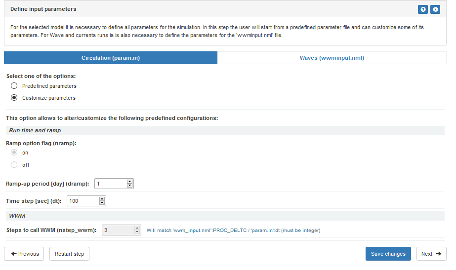
Figure 42 - Detail of the Outputs Viewer; Adding point to chart tool

Model Output Files

The user can see all available files, generated by the model, for all simulated days in a list by selecting the “Files” button/tab. As the list may be long, a search mechanism is implemented to facilitate the download. The download of each file can be done by clicking on the file name and just saving it to the user’s Downloads folder.

Figure 43 - Preview of the Outputs Viewer; focusing on the Files Feature

Online Demo

A live hands-on demo on the use of the 3 main features of OPENCoastS will be available soon.

Rating the service

Under the main menu (top right screen), a link to rate the OPENCoastS service is available. Users can grant up to 5 stars (1-bad to 5-excellent) and leave comments on his/her experience and suggestions to the development team. This feature aims to infer about users’ experience in order to improve the platform’s usability and functionality; also to receive feedback from users about their models’ outputs to infer about their quality. Therefore, the platform inquires users automatically one week after having their first deployment up and running. User’s ratings are saved and presented on this page.

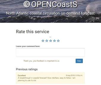
Figure 44 - OPENCoastS service Rating feature

Acknowledgements

The OPENCoastS service is one of the thematic services of the H2020 Research and Innovation programme EOSC-hub project, funded by European Union under grant agreement No. 777536.

This service takes advantage of many services and assets freely available online. We would like to acknowledge:

● NOAA and MeteoFrance – for the atmospheric predictions

● CMEMS - for the water level, salinity and temperature 3D predictions

● EMODnet Physics – for the publication of monitoring stations data

● FES2014 – for the global tide database

● SCHISM development team, in particular the lead developer, Prof. Joseph Zhang (from VIMS, USA).

The development team also acknowledges all colleagues that have helped to setup and test the several versions of the service.